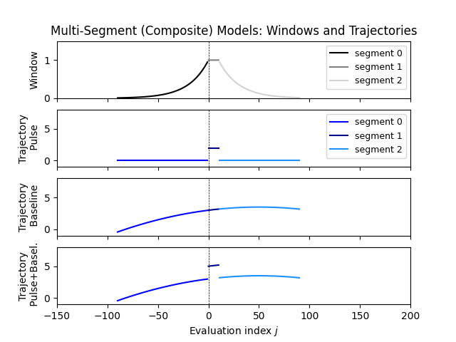
Multi-Segment (Composite) Models: Windows and Trajectories [ex104.0]

Defines a Composite Cost, consisting of two stacked ALSSM models, and applies them to detect pulses.

import matplotlib.pyplot as plt
import numpy as np
from scipy.signal import find_peaks

import lmlib as lm
from lmlib.utils.generator import (gen_rand_pulse, gen_wgn, gen_rand_walk)


# Defining ALSSM models
alssm_pulse = lm.AlssmPoly(poly_degree=0, label="line-model-pulse")
alssm_baseline = lm.AlssmPoly(poly_degree=2, label="offset-model-baseline")

# Defining segments with a left- resp. right-sided decaying window and a center segment with nearly rectangular window
semgent_left = lm.Segment(a=-np.inf, b=-1, direction=lm.FORWARD, g=20)
semgent_center= lm.Segment(a=0, b=10, direction=lm.FORWARD, g=5000)
semgent_right = lm.Segment(a=10+1, b=np.inf, direction=lm.BACKWARD, g=20, delta=10)

# Defining the final cost function
# mapping matrix between models and segments (rows = models, columns = segments)
F = [[0, 1, 0],
     [1, 1, 1]]

costs = lm.CompositeCost((alssm_pulse, alssm_baseline), (semgent_left, semgent_center, semgent_right), F)
x0 = [2, 3, 0.02, -0.0002] # initial states of alssm_pulse [0:1] and of alssm_baseline [1:4]

windows = costs.windows(segment_indices=[0,1,2], thd=0.01)


F_baseline_only = [[0, 0, 0],
                   [1, 1, 1]]
F_pulse_only    = [[0, 1, 0],
                   [0, 0, 0]]

trajecotries_baseline = costs.trajectories([x0], F_baseline_only, thd=0.01)
trajecotries_pulse = costs.trajectories([x0], F_pulse_only, thd=0.01)
trajecotries = costs.trajectories([x0], F, thd=0.01)

fig, axs = plt.subplots(4, sharex='all')

# Plot Window
for (js, weights), loc, c in zip(windows, ('0', '1', '2'), ('black','gray','lightgray')):
    axs[0].plot(js, weights, c=c, lw=1.5, label=f'segment {loc}')
axs[0].axvline(0, color="black", linestyle="--", lw=0.5)
axs[0].set_ylabel('Window')
axs[0].set_ylim([-0, 1.5])
axs[0].legend(fontsize=9)


# Plot Trajectory Pulse
for (js, trajs), loc, c in zip(trajecotries_pulse[0], ('0', '1', '2'), ('blue','darkblue','dodgerblue')):
    axs[1].plot(js, trajs, lw=1.5, c=c, label=f'segment {loc}')
axs[1].axvline(0, color="black", linestyle="--", lw=0.5)
axs[1].set_ylabel('Trajectory\n Pulse')
axs[1].set_ylim([-1, 8.0])
axs[1].legend(fontsize=9)

# Plot Trajectory Baseline
for (js, trajs), loc, c in zip(trajecotries_baseline[0], ('0', '1', '2'), ('blue','darkblue','dodgerblue')):
    axs[2].plot(js, trajs, lw=1.5, c=c)
axs[2].axvline(0, color="black", linestyle="--", lw=0.5)
axs[2].set_ylabel('Trajectory\n Baseline')
axs[2].set_ylim([-1, 8.0])

# Plot Trajectory Pulse+Baseline
for (js, trajs), loc, c in zip(trajecotries[0], ('0', '1', '2'),  ('blue','darkblue','dodgerblue')):
    axs[3].plot(js, trajs, lw=1.5, c=c)

axs[3].axvline(0, color="black", linestyle="--", lw=0.5)
axs[3].set_ylabel('Trajectory\n Pulse+Basel.')
axs[3].set_ylim([-1, 8.0])

axs[-1].set_xlabel('Evaluation index $j$')
axs[0].set_title('Multi-Segment (Composite) Models: Windows and Trajectories')

axs[0].set_xlim([-150, 200])
plt.show()

previous

Single-Segment (CostSegment) Models: Trajectories and Windows [ex103.0]

next

Local Signal Approximation and Trajectories [ex105.0]