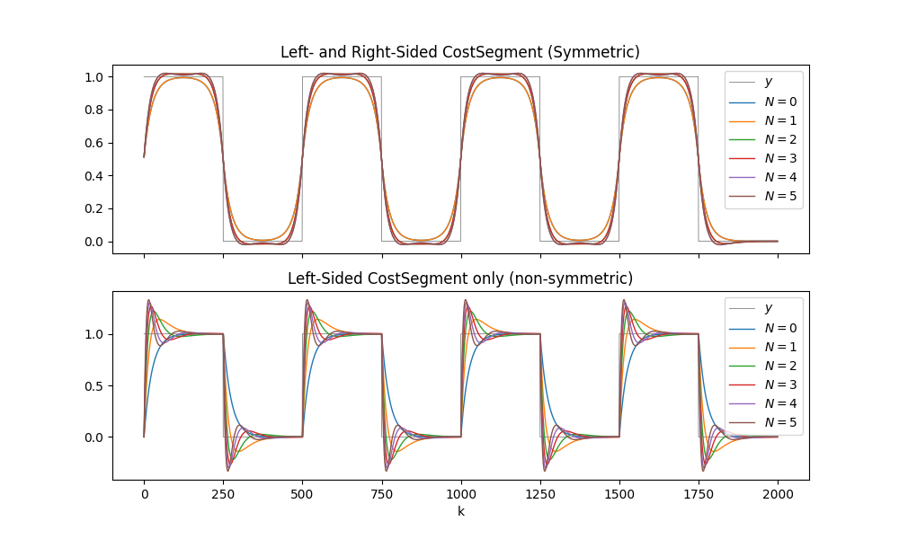
Symmetric and Non-Symmetric Polynomial Filters with ALSSMs [ex122.0]

Applies Composite Costs of polynomials of degrees N=0..6.

Out:

Badly Conditioned Steady State Matrix W: Use larger boundaries or lower g.
Badly Conditioned Steady State Matrix W: Use larger boundaries or lower g.
Badly Conditioned Steady State Matrix W: Use larger boundaries or lower g.
Badly Conditioned Steady State Matrix W: Use larger boundaries or lower g.
Badly Conditioned Steady State Matrix W: Use larger boundaries or lower g.
Badly Conditioned Steady State Matrix W: Use larger boundaries or lower g.
Badly Conditioned Steady State Matrix W: Use larger boundaries or lower g.
Badly Conditioned Steady State Matrix W: Use larger boundaries or lower g.

import matplotlib.pyplot as plt
import numpy as np
import lmlib as lm
from lmlib.utils.generator import gen_rect
import time

# --- Generating test signal ---
K = 2000
k = np.arange(K)
y = gen_rect(K, 500,250)


# --- ALSSM Filtering ---
y_hats_sym = []
y_hats_left = []

for i in range(0,6):
    # Polynomial ALSSM
    alssm_poly = lm.AlssmPoly(poly_degree=i)

    # Segments
    segment_left = lm.Segment(a=-np.inf, b=-1, direction=lm.FORWARD, g=25)
    segment_right = lm.Segment(a=0, b=np.inf, direction=lm.BACKWARD, g=25)

    # -- Symmetric Filter --
    # CompsiteCost
    costs = lm.CompositeCost((alssm_poly,), (segment_left, segment_right), F=[[1, 1]])

    # filter signal and take the approximation
    rls = lm.create_rls(costs, steady_state=True)
    xs = rls.filter_minimize_x(y)

    # extracts filtered signal
    y_hats_sym.append(costs.eval_alssm_output(xs, alssm_weights=[1]))


    # -- Left-Sided Filter --
    # CompsiteCost
    costs = lm.CompositeCost((alssm_poly,), (segment_left, segment_right), F=[[1, 0]])

    # filter signal and take the approximation
    rls = lm.create_rls(costs, steady_state=True)
    xs = rls.filter_minimize_x(y)

    # extracts filtered signal
    y_hats_left.append(costs.eval_alssm_output(xs, alssm_weights=[1]))


# --- Plotting ----
STYLES = ['tab:blue','tab:orange','tab:green','tab:red','tab:purple','tab:brown']
fig, ax = plt.subplots(2, sharex='all', figsize=(10,6))
ax[0].plot(k, y, lw=0.6, c='gray', label=rf'$y$')
for (i, y_hat) in enumerate(y_hats_sym):
   ax[0].plot(k, y_hat, STYLES[i], lw=1, label=r'$N='+str(i)+'$')
ax[0].legend(loc='upper right')
ax[0].set_title('Left- and Right-Sided CostSegment (Symmetric)')

ax[1].plot(k, y, lw=0.6, c='gray', label=rf'$y$')
for (i, y_hat) in enumerate(y_hats_left):
   ax[1].plot(k, y_hat, STYLES[i], lw=1, label=r'$N='+str(i)+'$')
ax[1].legend(loc='upper right')
ax[1].set_title('Left-Sided CostSegment only (non-symmetric)')
ax[1].set_xlabel('k')

plt.show()

previous

Symmetric Moving Average Filters with ALSSMs [ex121.0]

next

Multi-Channel Symmetric Signal Filter [ex123.0]