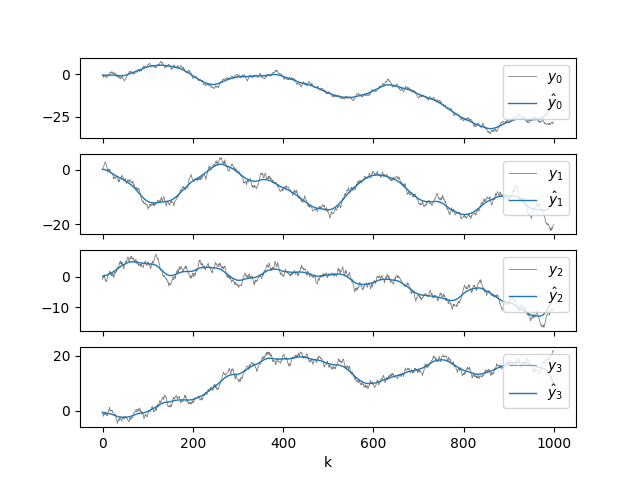
Multi-Channel Symmetric Signal Filter [ex123.0]

Applies a Composite Cost with a symmetric window as a symmetric, linear filter to a multi-channel signal.

import matplotlib.pyplot as plt
import numpy as np
import lmlib as lm
from lmlib.utils.generator import gen_rand_walk

# --- Generating test signal ---
K = 1000
seeds = [130, 150, 200, 220]
y = np.column_stack([gen_rand_walk(K, seed=s) for s in seeds])

# --- ALSSM Filtering ---
# Polynomial ALSSM
alssm_poly = lm.AlssmPoly(poly_degree=3)

# Segments
segment_left = lm.Segment(a=-np.inf, b=0, direction=lm.FW, g=20)
segment_right = lm.Segment(a=1, b=np.inf, direction=lm.BW, g=20)

# CompsiteCost
costs = lm.CompositeCost((alssm_poly,), (segment_left, segment_right), F=[[1, 1]])

# filter signal and take the approximation
rls = lm.create_rls(costs, multi_channel_set=True, steady_state=True)
xs = rls.filter_minimize_x(y)

# extracts filtered signals
y_hat = costs.eval_alssm_output(xs, alssm_weights=[1])

# --- Plotting ----
fig, axs = plt.subplots(len(seeds), 1, sharex='all')
for m, ax in enumerate(axs):
    ax.plot(y[:, m], lw=0.6, c='gray', label=r'$y_{}$'.format(m))
    ax.plot(y_hat[:, m], lw=1, label=r'$\hat{{y}}_{}$'.format(m))
    ax.legend(loc='upper right')

axs[-1].set_xlabel('k')

plt.show()

previous

Symmetric and Non-Symmetric Polynomial Filters with ALSSMs [ex122.0]

next

(Edu) Edge Detection [ex401.0]