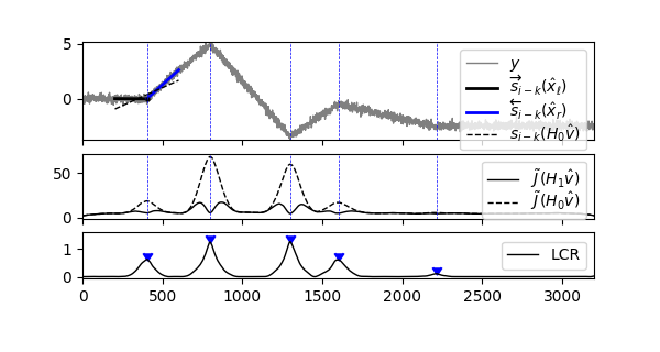
Edge Detection [ex401.1]

Example published in [Waldmann2022] as Example 1.

This basic example illustrates the detection of edges using a Two-Sided Line Model (TSLM), weighting the two options of a “Continuous” versus a “Straight” line in a LCR term.

import numpy as np
import matplotlib.pyplot as plt
from scipy.signal import find_peaks

import lmlib as lm
from lmlib.utils.generator import gen_slopes, gen_wgn



# --- Generate Test Signal ---
fs = 1         # (Relative) Sampling rate
K = 3200 * fs    # Length of Test signal
k = range(K)
ks = np.multiply([400, 800, 1300, 1600, 2200],fs)
deltas = [0, 5, -8.5, 3, -2]
y = gen_slopes(K, ks, deltas) + 1.0 * gen_wgn(K, sigma=0.2, seed=3141)


# 0 -- Parameters -----
a   = (-200*fs)    # Left segment length
b   = (200*fs) -1  # Right segment length
gl  = 70.0 * fs    # Left segment window decay
gr  = 70.0 * fs    # Right segment window decay


# 1 -- Two-Sided Line Model (TSLM)-----

# cost model to detect events
ccost = lm.TSLM.create_cost( ab=(a, b), gs=(gl, gr) )

# the following two costs are for visulatization purpose only - and not needed to solve the problem
cost_l = lm.TSLM.create_cost( ab=(a, 0), gs=(gl, gr) )
cost_r = lm.TSLM.create_cost( ab=(-1, b), gs=(gl, gr) )

# Applying Filters
separam = lm.RLSAlssm(ccost)
separam.filter(y)

separam_l = lm.RLSAlssmSteadyState(cost_l)
separam_l.filter(y)
separam_r = lm. RLSAlssmSteadyState(cost_r)
separam_r.filter(y)

# Filter
x_hat_line = separam.minimize_x(lm.TSLM.H_Straight)
x_hat_edge_l = separam_l.minimize_x()
x_hat_edge_r = separam_r.minimize_x()
x_hat_edge = separam.minimize_x(lm.TSLM.H_Continuous)

# Square Error and LCR
error_edge_l = separam_l.eval_errors(x_hat_edge_l)
error_edge_r = separam_r.eval_errors(x_hat_edge_r)
error_edge   = separam.eval_errors(x_hat_edge)
error_line   = separam.eval_errors(x_hat_line)
lcr = -1 / 2 * np.log(np.divide(error_edge, error_line))


# Find LCR peaks with minimal distance and height
peaks_1, _ = find_peaks(lcr, height=.1, distance= 200*fs)

# Evaluate trajectories (for plotting only)
trajs_edge = lm.map_trajectories(ccost.trajectories(x_hat_edge[peaks_1]), peaks_1, K, merge_ks=False)
trajs_line = lm.map_trajectories(ccost.trajectories(x_hat_line[peaks_1]), peaks_1, K, merge_ks=False)

wins = lm.map_windows(ccost.windows(segment_indices=[1, 1]), peaks_1, K, merge_ks=True)


# -- PLOTTING --
_, axs = plt.subplots(3, 1, figsize=(6, 3.2), gridspec_kw={'height_ratios': [1.5, 1.0, 0.7]}, sharex='all')
nax = 0 # current subplot index

t = np.array(list(k))
axs[nax].plot(t, y, lw=1, c='gray', label='$y$', zorder=0)
for index in range(peaks_1.shape[0]): # iterate through the peaks
   axs[nax].plot(t, trajs_edge[index, 0, :], c='k', lw=2, ls='-', zorder=1, label='$\overrightarrow{s}_{i-k}(\hat x_\ell)$')
   axs[nax].plot(t, trajs_edge[index, 1, :], c='b', lw=2, ls='-', zorder=1, label='$\overleftarrow{s}_{i-k}(\hat x_r)$')
   axs[nax].plot(t, trajs_line[index, 0, :], c='k', lw=1, ls='--', zorder=1, label='${s}_{i-k}(H_0 \hat v)$')
   axs[nax].plot(t, trajs_line[index, 1, :], c='k', lw=1, ls='--', zorder=1)
   axs[nax].scatter(peaks_1[0], x_hat_edge[peaks_1[0], 0], marker='.', c='k', s=20.0)

   break # only show trajectory of the first peak (comment out to show all trajectories)

for xp in peaks_1:
   axs[nax].axvline(x=xp, ls='--', c='b', lw=0.5)

axs[nax].legend(loc='upper right', labelspacing = -0.0)
axs[nax].set_ylim(bottom=min(y),top=max(y))
nax+=1

# Cost plot
kswitch=ks[1]
kdif=ks[1]-kswitch
axs[nax].plot(k, error_edge, c='xkcd:black', label=r'$\tilde J(H_1 \hat v)$', lw=1.0)
axs[nax].plot(k, error_line, c='xkcd:black', ls='--',label=r'$\tilde J(H_0 \hat v)$', lw=1.0)

axs[nax].legend(loc='upper right', labelspacing = -0.0)
for xp in peaks_1:
   axs[nax].axvline(x=xp, ls='--', c='b', lw=0.5)

nax+=1
# LCR plot
axs[nax].plot(k, np.concatenate((lcr[kdif:],lcr[0:kdif],)), c='xkcd:black', label='LCR', lw=1.0)
axs[nax].legend(loc='center right')
axs[nax].scatter(peaks_1, lcr[peaks_1], marker=7, c='b')
axs[nax].set_ylim(-0.05, 1.6)
axs[nax].set_xlim(left=0.0, right=3200.0)

plt.subplots_adjust(bottom=0.21)


plt.show()

previous

(Edu) Edge Detection [ex401.0]

next

Notch Detection in ABP Signal [ex402.0]