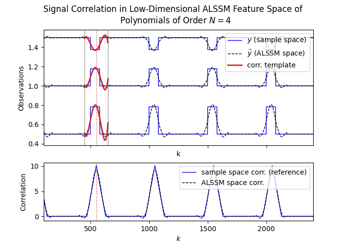
Correlation/Convolution in Low-Dimensional ALSSM Feature Space [ex501.0]

Performs correlation (or convolution) of a multi-channel signal (blue) with a given template (red) in a low dimensional ALSSM feature space. Correlation a lower dimensonal space is in many cases faster than the direct correlation in the high-dimensional sample space.

Author(s): Christof Baeriswyl

Out:

Processing Speed Measurements
-----------------------------
Duration of correlation (or convolution) in ALSSM feature space (w/o mapping time):      0.041ms
Duration of correlation (or convolution) in sample space.                        :      8.821ms

import numpy as np
import matplotlib.pyplot as plt
from matplotlib import gridspec
import time
import lmlib as lm
from lmlib.utils.generator import gen_rect
from lmlib.utils.generator import gen_wgn
from lmlib.utils.generator import gen_conv


# -- 0. Generate Test signal ---
K = 2500  # number of samples to process
k = range(K)
NOFCH = 3 # number of channels
K_REF = 550 # Location of reference template (Index of shape to correlate with)
y_mc = np.outer(gen_rect(K, 500, 80)*.2, -gen_wgn(NOFCH, 1.0, seed=156789)) # Generate Test signal.

# -- 1. Polynomial ALSSM model for later signal approximation --
a = -100 # length of shape to correlate with, i.e., uses samples {K_REF+a, ..., K_REF+b} as the correlation template
b = 100
N = 4  # polynomial order (number of coefficients)
alssm = lm.AlssmPolyJordan(poly_degree=N, label='Alssm')
segment = lm.Segment(a=a, b=b, direction=lm.BACKWARD, g=400)
cost = lm.CostSegment(alssm, segment)

# -- 2. Project observations (and the template) to ALSSM feature space --
rls_y = lm.create_rls(cost, multi_channel_set=True)
rls_y.filter(y_mc) # Transform observations

xs_hat = rls_y.minimize_x() # get transformed observations
xs_h = xs_hat[K_REF] # get correlation tempalte

y_hat = cost.eval_alssm_output(xs_hat) # signal reconstruction using ALSSM approximation (for illustration only)





# -- 3. Fast convolution in ALSSM feature space (channel-wise) --
print("Processing Speed Measurements")
print("-----------------------------")


start = time.process_time() # start timer for speed comparison

corr_alssm = np.zeros(K)
for j in range(NOFCH):
    corr_alssm = corr_alssm + np.matmul(rls_y.xi[:,:,j], xs_h[:,j])

print("Duration of correlation (or convolution) in ALSSM feature space (w/o mapping time): {:10.3f}ms".format((time.process_time()-start)*1e3))


# -- 4. Standard convolution in sample space (channel-wise) (for comparison) --
start = time.process_time() # start timer for speed comparison

corr_native = np.zeros(y_mc.shape[0])
h_mc = y_mc[K_REF+a:K_REF+b+1,:] # cut out impulse response
for j in range(NOFCH):
    corr_native[-a:-a+K-(b-a)] += np.correlate(y_mc[:,j], h_mc[:,j], 'valid')

print("Duration of correlation (or convolution) in sample space.                        : {:10.3f}ms".format((time.process_time()-start)*1e3))



# -- 5.  Plotting --
template_trajectory = lm.map_trajectories(cost.trajectories([xs_h,]), [K_REF,] , K,
                                     merge_ks=True, merge_seg=True)

_, axs = plt.subplots(2, 1, figsize=(7, 5), gridspec_kw={'height_ratios': [2, 1]}, sharex='all')
nax = 0
offsets = (np.arange(NOFCH, 0, -1)*.5)

# Observation
axs[nax].set(xlabel='k', ylabel=r'$y$')
axs[nax].plot(k, y_mc + offsets, c='b', lw=1, label=['$y$ (sample space)', '', ''])
axs[nax].plot(k, y_hat + offsets, c='k', linestyle="--", lw=1, label=['$\hat y$ (ALSSM space)', '', ''])
axs[nax].plot(k, template_trajectory + offsets,'-' , c='tab:red', lw=2.0, label=['corr. template', '', ''])
axs[nax].axvline(K_REF+a, color="black", linestyle="--", lw=0.5)
axs[nax].axvline(K_REF+b, color="black", linestyle="--", lw=0.5)
axs[nax].axvline(K_REF, color="tab:red", linestyle=":", lw=1.0)
axs[nax].legend(loc='upper right')
axs[nax].set(ylabel='Observations')
ch_labels = ['Obs. CH {}'.format(i) for i in range(NOFCH,0,-1)]
# axs[nax].legend(ch_labels)

# Convolution
nax+=1
axs[nax].set(xlabel='$k$')
axs[nax].plot(k, corr_native, c='b', lw=1, linestyle='-', label="sample space corr. (reference)")
axs[nax].plot(k, corr_alssm, '--', c='k', lw=1, label="ALSSM space corr.")
axs[nax].axvline(K_REF, color="tab:red", linestyle=":", lw=1.0)
axs[nax].legend(loc='upper right')
axs[nax].set(ylabel='Correlation')

axs[nax].set_xlim(100, K-100)

plt.suptitle('Signal Correlation in Low-Dimensional ALSSM Feature Space of \n Polynomials of Order $N='+str(N)+'$')
plt.show()

previous

ECG Shape Detection [ex113.0]

next

Matched Filter in Low-Dimensional ALSSM Feature Space [ex502.0]