Note
Click here to download the full example code
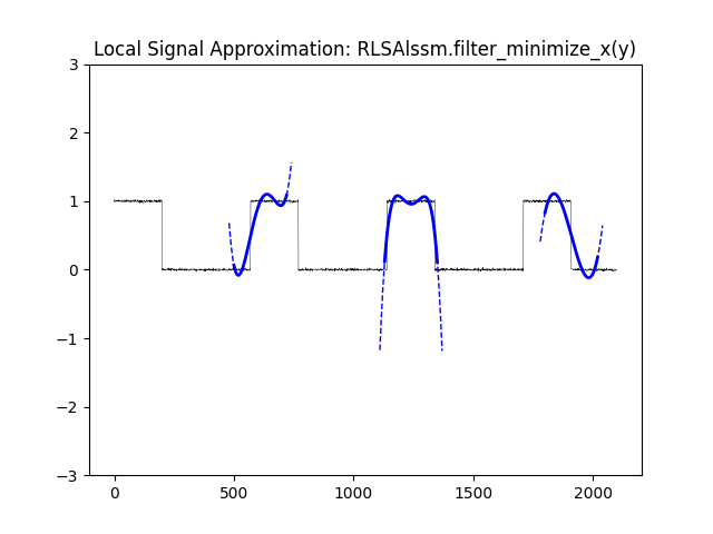
Local Signal Approximation and Trajectories [ex105.0]#
Local Signal Approximation and Trajectories using PolyAlssm.
Out:
Badly Conditioned Steady State Matrix W: Use larger boundaries or lower g.
import matplotlib.pyplot as plt
import lmlib as lm
import numpy as np
from lmlib.utils.generator import gen_wgn, gen_rect

K = 2100
y = gen_rect(K, 570, 200) + gen_wgn(K, 0.01)

cost = lm.CostSegment(lm.AlssmPoly(poly_degree=4),
                      lm.Segment(0, 220, lm.BW, 300))
cost_wide = lm.CostSegment(lm.AlssmPoly(poly_degree=4),
                      lm.Segment(0-20, 220+20, lm.BW, 300))

rls = lm.RLSAlssmSteadyState(cost) # Using steady state leads to faster computation and increased nummerical stability
xs = rls.filter_minimize_x(y)

K_refs = [500, 1130, 1800]
trajs = lm.map_trajectories(cost.trajectories(xs[K_refs], thd=0.01), K_refs, K, merge_ks=True, merge_seg=True)
trajs_wide = lm.map_trajectories(cost_wide.trajectories(xs[K_refs], thd=0.01), K_refs, K, merge_ks=True, merge_seg=True)

plt.title('Local Signal Approximation: RLSAlssm.filter_minimize_x(y)')
plt.plot(y, lw=0.3, c='k', label='y')
plt.plot(trajs, lw=2, c='b', label='y_hat')
plt.plot(trajs_wide, lw=1, ls='--', c='b', label='y_hat')
plt.ylim([-3, 3])

plt.show()
Total running time of the script: ( 0 minutes 0.117 seconds)